
Bird Species Not Found
Please return to the Climate Change Bird Atlas page and search for another bird species.
Last Modified: March 28, 2019
Please return to the Climate Change Bird Atlas page and search for another bird species.
Last Modified: March 28, 2019
This tool allows you to compare two species side-by-side. Select a species to display as the "Left Image" using the menu, and a species to display as the "Right Image."
 Click and drag the orange handle over the maps to compare.
Percent Area Occupied simply is the percent of 20x20 km cells within the total area of the eastern United States that have been modeled to be suitable for the species. There are a total of 9767 cells used in the model.
Ave. IV is the average importance value across all 20x20 km cells that have been modeled to be suitable for the species.
Sum IV is the sum of importance values across all cells. Thus it is a metric that considers both the abundance and the range of the species, perhaps the best metric of overall species importance.
")
 of the species as calculated from the BBS data. The BBS Incidence (on a scale of 0 – 1) represents the proportion of times a species was observed on a route over a decade.")
This tool allows you to compare two predictor variables side-by-side. Select a predictor variable to display as the "Left Image" using the menu, and a predictor variable to display as the "Right Image."
If you select a Climate predictor variable, you can also select the climate scenario (e.g. HadleyCM3 – A1FI (High, "Harsh") or Current) as well.
Click and drag the orange handle over the maps to compare.
 HadleyCM3 – A1FI (High,")
 Current Modelled")
Boxplots provide a quick visual of the distribution of the variable importance from the random forest models from all 147 species (black boxplot) and how each species fits into the overall distribution (cyan line). The box encompasses from the 25th to the 75th percentile of the data. The thick line within the box identifies the median (50th percentile). The whiskers extend 1.5 times the interquartile range (75th-25th). This shows the spread of the data. Data points that lay beyond this range are shown with circles. The first figure shows all 38 predictor variables together (numbers on the x-axis). By clicking on each group (climate, elevation, vegetation set1, vegetation set2, and vegetation set3) a plot of each group will be opened.
| Predictor | Predictor Code | Predictor Name | 1 | PPT | Annual precipitation (mm) | 2 | PPTMAYSEP | Mean May-September precipitation (mm) | 3 | TJAN | Mean January temperature (°C) | 4 | TJUL | Mean July temperature (°C) | 5 | JULJANDIFF | Mean difference between July and January Temperature (°C) | 6 | TMAYSEP | Mean May-September temperature (°C) | 7 | TAVG | Mean annual temperature (°C) | 8 | ELV_MIN | Minimum elevation (m) | 9 | ELV_MAX | Maximum elevation (m) | 10 | ELV_RANG | Range of elevation (m) | 11 | ELV_MEAN | Average elevation (m) | 12 | 12 | Distribution of balsam fir | 13 | 97 | Distribution of red spruce | 14 | 110 | Distribution of shortleaf pine | 15 | 111 | Distribution of slash pine | 16 | 126 | Distribution of pitch pine | 17 | 129 | Distribution of eastern white pine | 18 | 131 | Distribution of loblolly pine | 19 | 261 | Distribution of eastern hemlock | 20 | 316 | Distribution of red maple | 21 | 318 | Distribution of sugar maple | 22 | 371 | Distribution of yellow birch | 23 | 372 | Distribution of sweet birch | 24 | 375 | Distribution of paper birch | 25 | 462 | Distribution of hackberry | 26 | 491 | Distribution of flowering dogwood | 27 | 531 | Distribution of American beech | 28 | 541 | Distribution of white ash | 29 | 611 | Distribution of sweetgum | 30 | 621 | Distribution of yellow-poplar | 31 | 693 | Distribution of blackgum | 32 | 746 | Distribution of quaking aspen | 33 | 762 | Distribution of black cherry | 34 | 802 | Distribution of white oak | 35 | 832 | Distribution of chestnut oak | 36 | 833 | Distribution of northern red oak | 37 | 835 | Distribution of post oak | 38 | 972 | Distribution of American elm |
|---|
Variable importance scores for this species is plotted in cyan and can be compared to all species importance scores which are plotted as boxplots. Thus for example, if the cyan line extends above the boxplot (or the median of the boxplot,shown as the bold black line), it indicates that the variable for that particular species is a more important predictor than for most of the other species.
If you click on one grouping of the plot (e.g., climate, elevation, etc), you will get a higher resolution image of that section of the plot.

| Predictor | Predictor Name | 1 | Annual precipitation (mm) | 2 | Mean May-September precipitation (mm) | 3 | Mean January temperature (°C) | 4 | Mean July temperature (°C) | 5 | Mean difference between July and January Temperature (°C) | 6 | Mean May-September temperature (°C) | 7 | Mean annual temperature (°C) | 8 | Minimum elevation (m) | 9 | Maximum elevation (m) | 10 | Range of elevation (m) | 11 | Average elevation (m) | 12 | Distribution of balsam fir | 13 | Distribution of red spruce | 14 | Distribution of shortleaf pine | 15 | Distribution of slash pine | 16 | Distribution of pitch pine | 17 | Distribution of eastern white pine | 18 | Distribution of loblolly pine | 19 | Distribution of eastern hemlock | 20 | Distribution of red maple | 21 | Distribution of sugar maple | 22 | Distribution of yellow birch | 23 | Distribution of sweet birch | 24 | Distribution of paper birch | 25 | Distribution of hackberry | 26 | Distribution of flowering dogwood | 27 | Distribution of American beech | 28 | Distribution of white ash | 29 | Distribution of sweetgum | 30 | Distribution of yellow-poplar | 31 | Distribution of blackgum | 32 | Distribution of quaking aspen | 33 | Distribution of black cherry | 34 | Distribution of white oak | 35 | Distribution of chestnut oak | 36 | Distribution of northern red oak | 37 | Distribution of post oak | 38 | Distribution of American elm |
|---|

| Predictor | Importance Value | PPT | PPTMAYSEP | TJAN | TJUL | JULJANDIFF | TMAYSEP | TAVG |
|---|

| Predictor | Importance Value | ELV_MIN | ELV_MAX | ELV_RANG | ELV_MEAN |
|---|

| Predictor | Importance Value | 12 | 97 | 110 | 111 | 126 | 129 | 131 | 261 |
|---|

| Predictor | Importance Value | 316 | 318 | 371 | 372 | 375 | 462 | 491 | 531 |
|---|

| Predictor | Importance Value | 621 | 693 | 746 | 762 | 802 | 832 | 833 | 835 | 972 |
|---|
Potential Changes in Abundance and Range (Future) |
||||
|---|---|---|---|---|
| GCM SCENARIO | % Area Occ | Ave IV | Sum IV | Future/Current IV |
This tool allows you to compare two climate models side-by-side. Select a scenario to display as the "Left Image" using the menu, and a scenario to display as the "Right Image."
Click and drag the orange handle over the maps to compare.
Percent Area Occupied simply is the percent of 20x20 km cells within the total area of the eastern United States that have been modeled to be suitable for the species. There are a total of 9767 cells used in the model.
Ave. IV is the average importance value across all 20x20 km cells that have been modeled to be suitable for the species.
Sum IV is the sum of importance values across all cells. Thus it is a metric that considers both the abundance and the range of the species, perhaps the best metric of overall species importance.
Future/Current IV is the ratio of change between the modeled current Sum IV and any of the GCM scenarios Sum IV.
")

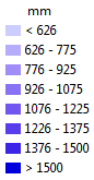
The Geographic Predictors Maps are derived from Regression Tree Analysis, where each terminal node of the 'tree' corresponds to a legend and map color that is represented on the map. As such, one can determine what variables may be driving the species' distribution and abundance at a particular part of its range. For example, a precipitation variable may determine the western boundary and a temperature variable may determine the northern boundary for a species. Also note that variables important high in the tree diagram relate to larger portions of the species' range, while those variables lower (closer to the terminal nodes) relate to more localized variables driving the distribution.
IMPORTANT: It is important to note that if the model reliability is NOT high for the species, then the confidence that the predictors in a single regression tree are driving the distribution is LOW. It is therefore worthwhile to compare the predictor importance according to the RandomForest model. In the species page, click the "Statistics, Tables & Interpretations" button in the "Current Distriubtion" panel for viewing the predictor importance table under RandomForest model.
NOTE: Example: If tavg >
< 6.5 means that if tavg> 6.5 deg C, traverse the left branch and if tavg
< 6.5 deg C traverse the right branch.
If tavg
<> 6.5 means that if tavg is less than 6.5, traverse the left branch. and if tavg > 6.5 traverse the right branch.
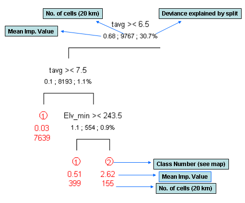
The regression-tree diagram along with the corresponding class-map shows what predictors are driving the distribution for this species.

